
Time Series Analysis
Analyzing Dynamic Load Profile Data (DLP) from Southern California Edison (SCE)
The goal of this challenge is to make use of public data (SCE DLP) and practice time series analysis. We will be looking at the average residential customer in SCE territory using R as our analysis software.
Load SCE Dynamic Load Profile Data from 1998 to 2015, merge these individual files, and export as csv for future reference.
setwd("~/Code/R/SCE")

library(RCurl)

#Load all the SCE DLP data from 1998 to 2015 and merge into one data frame

Y98 <- getURL("https://www.sce.com/005_regul_info/eca/DOMSM98.DLP")
Y98 <- read.csv(text = Y98)
Y99 <- getURL("https://www.sce.com/005_regul_info/eca/DOMSM99.DLP")
Y99 <- read.csv(text = Y99)
Y00 <- getURL("https://www.sce.com/005_regul_info/eca/DOMSM00.DLP")
Y00 <- read.csv(text = Y00)

Y01 <- getURL("https://www.sce.com/005_regul_info/eca/domsm01.dlp")
Y01 <- read.csv(text = Y01)
Y02 <- getURL("https://www.sce.com/005_regul_info/eca/DOMSM02.DLP")
Y02 <- read.csv(text = Y02)
Y03 <- getURL("https://www.sce.com/005_regul_info/eca/DOMSM03.DLP")
Y03 <- read.csv(text = Y03)

Y04 <- getURL("https://www.sce.com/005_regul_info/eca/DOMSM04.DLP")
Y04 <- read.csv(text = Y04)
Y05 <- getURL("https://www.sce.com/005_regul_info/eca/DOMSM05.DLP")
Y05 <- read.csv(text = Y05)
Y06 <- getURL("https://www.sce.com/005_regul_info/eca/DOMSM06.DLP")
Y06 <- read.csv(text = Y06)

Y07 <- getURL("https://www.sce.com/005_regul_info/eca/DOMSM07.DLP")
Y07 <- read.csv(text = Y07)
Y08 <- getURL("https://www.sce.com/005_regul_info/eca/DOMSM08.DLP")
Y08 <- read.csv(text = Y08)
Y09 <- getURL("https://www.sce.com/005_regul_info/eca/DOMSM09.DLP")
Y09 <- read.csv(text = Y09)

Y10 <- getURL("https://www.sce.com/005_regul_info/eca/DOMSM10.DLP")
Y10 <- read.csv(text = Y10)
Y11 <- getURL("https://www.sce.com/005_regul_info/eca/DOMSM11.DLP")
Y11 <- read.csv(text = Y11)
Y12 <- getURL("https://www.sce.com/005_regul_info/eca/DOMSM12.DLP")
Y12 <- read.csv(text = Y12)

Y13 <- getURL("https://www.sce.com/005_regul_info/eca/DOMSM13.DLP")
Y13 <- read.csv(text = Y13)
Y14 <- getURL("https://www.sce.com/005_regul_info/eca/DOMSM14.DLP")
Y14 <- read.csv(text = Y14)
Y15 <- getURL("https://www.sce.com/005_regul_info/eca/DOMSM15.DLP")
Y15 <- read.csv(text = Y15)

Y98_15 <- rbind(Y98, Y99, Y00, Y01, Y02, Y03, Y04, Y05, Y06, Y07, Y08, Y09, Y10, Y11, Y12, Y13, Y14, Y15)

# Write CSV in R
write.csv(Y98_15, file = "Y98_15.csv")
Load the csv we just exported, process the Datetime signature, convert to an time-series object,
library(ggplot2)
library(xts)
library(forecast)

setwd("~/Code/R/SCE")

TimeS <- read.csv(file = "Y98_15.csv")

TimeS$Date <- as.Date(TimeS$Date, "%m%d%Y")

TimeS <- TimeS[,-c(1:3)]

#StartDate
TimeS$Date[1]
#04/01/98

#EndDate
TimeS$Date[6158]
#02/08/2015

#Setup the Date Time - remove trailing days in feb
time <- seq(from = as.POSIXct("1998-04-01 01:00"),
 to = as.POSIXct("2015-01-31 24:00"), by = "hour")
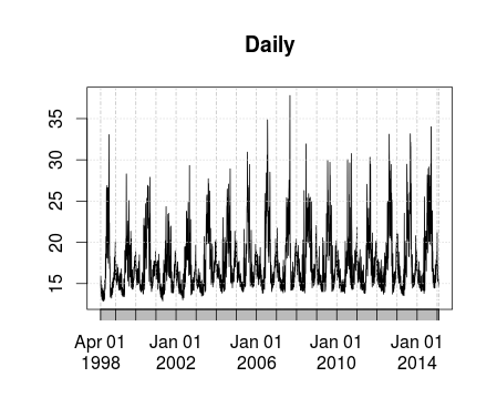
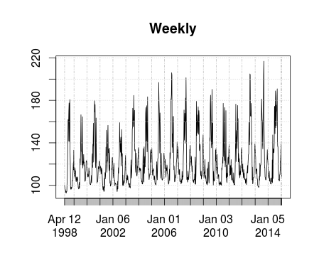
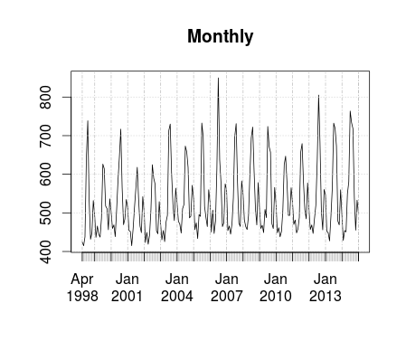
Lets look at the daily, weekly, monthly, and annual sums to get a first impression of trends and seasonality.
#Setup the Dependent Variable - remove trailing days in feb
kW <- as.vector(t((as.matrix(TimeS))))
kW <- kW[1:length(time)]
kW <- xts(kW, order.by=time, frequency = 12) #Frequency is guessed

Daily <- apply.daily(kW,sum)
Daily <- Daily[1:(length(Daily)-1)] # Remove Trailing hour

Weekly <- apply.weekly(kW,sum)
Weekly <- Weekly[1:(length(Weekly)-1)] # Remove Trailing Week
Weekly <- Weekly[2:length(Weekly)] # Remove Leading Week

Monthly <- apply.monthly(kW,sum)
Monthly <- Monthly[1:(length(Monthly)-1)] # Remove Trailing Month

Yearly <- apply.yearly(kW,sum)
Yearly <- Yearly[1:(length(Yearly)-1)] # Remove Trailing hour
Yearly <- Yearly[2:length(Yearly)] # Remove Leading Year

plot(Daily)
plot(Weekly)
plot(Monthly)
plot(Yearly)

Additive Decomposition Model: xt = mt + s t + z t
Multiplicative Decomposition Model: xt = mt · s t + z t
where:
xt is the observation
mt is the trend
s t is the seasonality
z t is the random residual
Decompose the hourly DLP using an additive model and a multiplicative model.
A multiplicative model is best used when the variance of the seasonality increases over time.
kW <- as.vector(t((as.matrix(TimeS))))
kW <- kW[1:length(time)]
kW <- ts(kW, start = c(1998, 4), end = c(2015,1),frequency = 8765)
kW.decomp <- decompose(kW)
kW.decomp.mult <- decompose(kW, type = "mult")
plot(kW.decomp)
plot(kW.decomp.mult)
trend <- kW.decomp$trend
Seasonal <- kW.decomp$seasonal


To get a better understanding if the variance of the seasonality is increasing overtime we can plot the average annual variance of the de-trended kW draw over time
MultTrend <- kW.decomp.mult$trend
MultSeason <- kW.decomp.mult$seasonal
MultRand <- kW.decomp.mult$random

SepYears <- split(Seasonal, cut(Monthly, 17))
VarOverTime <- sapply(SepYears, var)
reg1 <- lm(VarOverTime~c(1:17))
plot(VarOverTime, main = "Annual Variance of Detrended Average Monthly kW draw")
abline(reg1)
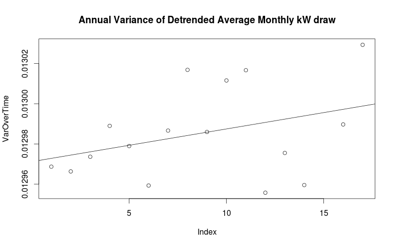
It appears that the variance of de-trended annual consumption is increasing over time and a multiplicative decomposition model might be optimal.
Lets inspect for hourly auto-correlation of the data after we’ve removed the trend and seasonality leaving just the random residual. We do this using a correlelogram.
MultRand <- na.rm
acf(MultRand[4383:144621])
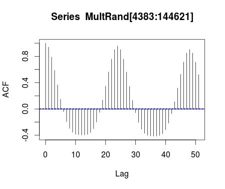

The x axis is in units of hours in this chart. We can see a 24 hour auto-correlation for consumption that may be decreasing over time.
Lets see if there is daily auto-correlation.
RandDecompDaily <- xts(MultRand[4383:144621], order.by=time[4383:144621], frequency = 24) #Frequency is guessed
RandDecompDaily <- apply.daily(RandDecompDaily,sum)
DailyConsump <- sapply(SepDays, sum)
acf(DailyConsump)

There is a high degree of daily auto-correlation.
Forecast using the Holt-Winters multiplicative method
Exponentially weighted averages
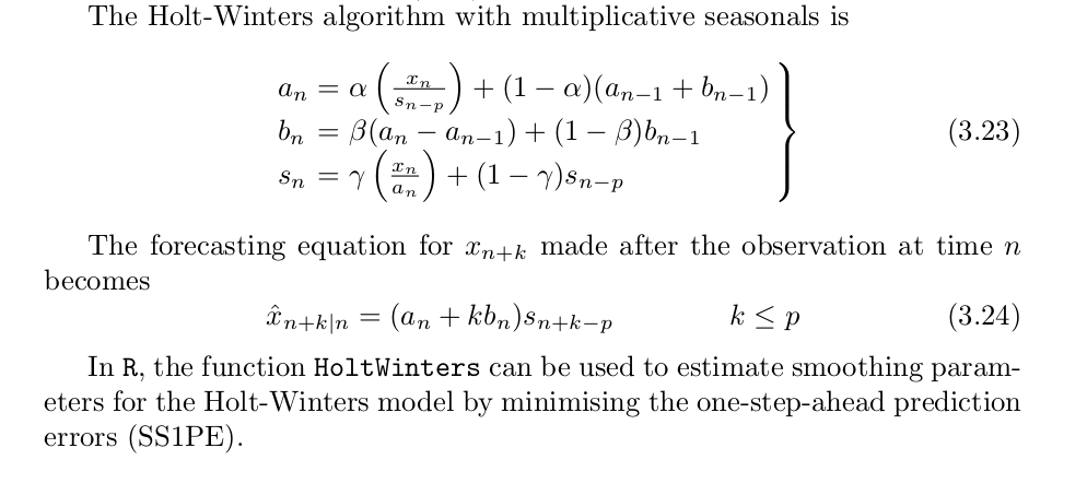 Source: Cowpertwait, Metcalfe
MonthlyNum = data.matrix(as.data.frame(Monthly))

MonthlyTs <- ts(MonthlyNum, start = c(1998, 4), end = c(2015,1),frequency = 12)
MonthlyTs.hw <- HoltWinters (MonthlyTs, seasonal = "mult")
MonthlyTs.hw; MonthlyTs.hw$coef; MonthlyTs.hw$SSE

plot(MonthlyTs.hw$fitted, main = "Holt-Winters Multiplicative Model")
plot(MonthlyTs.hw, main = "Holt-Winters Seasonal Multiplicative Fit", ylab = "Monthly kWh Consumption")
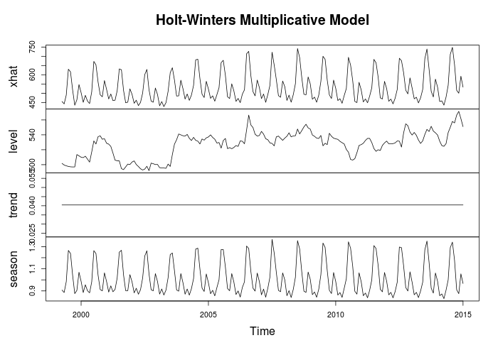

This is an in sample fit. We are trying to create a best fit of our monthly kWh consumption. Let’s try and do a year ahead prediction using Holt-Winters
MonthlyTs.predict <- predict(MonthlyTs.hw, n.ahead = 12)
ts.plot(MonthlyTs, MonthlyTs.predict, lty = 1:2, main = "Holt-Winters Year Ahead Prediction", ylab = "Monthly kWh Consumption")

We need to assess how well our model is performing. A common metric is the mean square one step ahead error.
sqrt(MonthlyTs.hw$SSE/length(MonthlyTs))
sd(MonthlyTs)
Out:
33.90183
90.07376
The mean square one step ahead error is 34 vs. the standard deviation of 90 which is a significant improvement.
Lets grab those model weights from the Holt-Winters model with Multiplicative Decomposition
MonthlyTs.hw$alpha
MonthlyTs.hw$beta
MonthlyTs.hw$gamma
Out:
alpha
0.1904494
beta
0

gamma
0.3095831
Alpha, Beta, and Gamma are smoothing parameters that correspond to the level, slope, and seasonal variation. The Level and Seasonal variation adapts rapidly whereas the slope does not.
Deterministic Models – Day Ahead Modeling
Lets try and use a simple linear regression for day ahead modeling. As a diagnostic test let’s plot the autocorrelation of the residuals in order to see if there is systematic bias.
DailyNum = data.matrix(as.data.frame(Daily))
DailyTs <- ts(DailyNum, start = c(1998, 4), end = c(2015,1),frequency = 1) dates = seq(as.Date("1998-04-01"), by = "day", along = DailyTs)
DailyTs.lm <- lm(DailyTs ~ dates) acf(resid(DailyTs.lm), main = "Daily Autocorrelation")

Indeed we see in the correlelogram some autocorrelation in our residuals showing that our linear model is not fully capturing the signal. We can see traces of Weekend and Weekday behavior in this diagnostic. We can
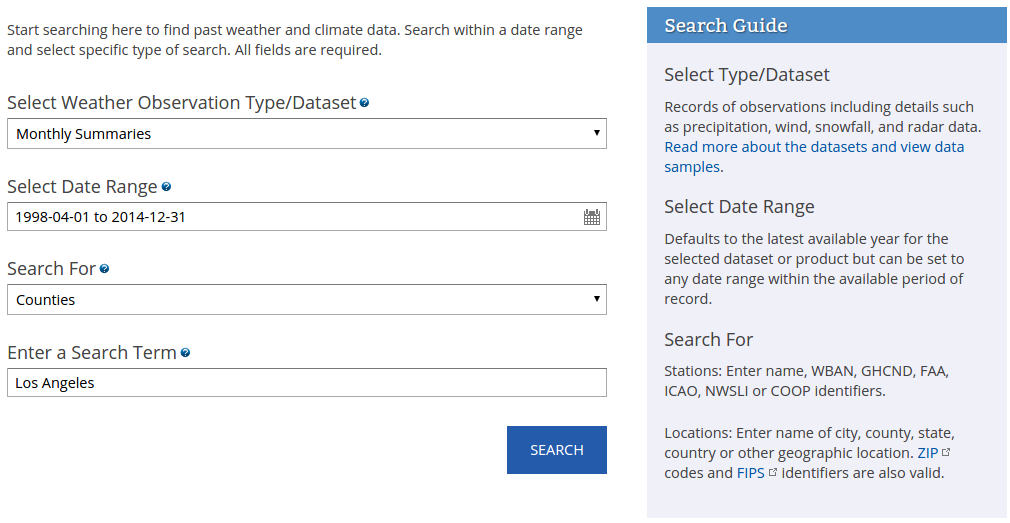
Future Next Steps (ENSO and CDD)
The Next step in this analysis is to download monthly cooling degree data from NOAA for Los Angeles County for the time period of interest 4/1998 to 12/2014.
http://www.ncdc.noaa.gov/cdo-web
______________________________________________________________________


Data Science London + Scikit Learn – 1/11/2015
See the documented code for this competition at my github page.
Here is the Kaggle competition page for this scikit learn oriented competition:
The goal of this competition is to familiarize users with the Scikit learn module in Python for Data Science and Prediction. During this competition (It had already expired but you can still submit entries) I conducted exploratory analysis, visualization, data pre-processing, regularization, resampling, and modeling all in Python. The goal was to accurately predict a logistic output using 40 features based on a training and test set.
I first checked for outliers, skewness, and multicolinearity before proceeding further because this will effect model performance. After centering and scaling my features (transforming the distribution was unnecessary) I then tried a few regularization techniques and ended up using Tree Selection and the Lasso method. I tried many different models using a 10 fold cross validation on my training data.
For more details and a step by step see the github page. Here were the results of the different model runs for this competition in ascending rank (you can submit multiple predictions):
| #Rank 115 with SVM and tree based selection (Same with or without scaling and centering) | |
| #Rank 176 with Random Forest and tree based selection | |
| #Rank 180 with Random Forest (No Regularization) | |
| #Rank 182 with logistic model and tree based selection | |
| #Rank 186 with lasso regression |
Mistakes and improvements: One interesting result was that scaling and centering my data provided no measurable improvements in my ranking with or without this pre-processing but this is a minor thing because it did not hurt performance. I found it interesting that during my 10 fold cross validation SVM did not outperform Random Forest so I would imagine that Random Forest would end up being my best model. However after I predicted the test data using the same regularization scheme as I did for Random Forest, SVM ended up winning by a large margin. Because the training set consisted of 1000 data points and the test data set consisted of 9000 test data points I might want to consider a resampling method other than 10-fold cross validation. For example I might want to do a repeated bootstrap resampling or a 50/50 split because my training set is much smaller compared to the test data set.
